
Full Steam Ahead: Mortal Engines for Linear Algebra
Two fields, each with a rich history, collide to make Thermodynamic Linear Algebra, providing the first theoretical speedups for Thermodynamic Computing


Our preprint Thermodynamic Linear Algebra, submitted on August 10th, drew a warm response from the broader tech community, stimulating thoughtful questions on Hacker News. Yann LeCun also apparently found it “Fun”, and some people started betting on a hardware implementation of our proposal.

This blog post will cover several highlights from the paper, including:
Novel thermodynamic algorithms for four different linear algebra primitives.
The first asymptotic scaling analysis for the thermodynamic computing paradigm, and the first theoretically predicted speedup for a thermodynamic algorithm.
The predicted speedups grow with the difficulty of the problem, i.e., with the matrix dimension and matrix condition number, and hence the speedups can be increased by considering more difficult problems.
Numerics with a detailed timing model for thermodynamic hardware, allowing comparison of predicted runtimes in practice, and indeed these numerics show that speedup is possible with realistic hardware in realistic situations.
A fundamental relation that captures the tradeoff between energy and time in algorithmic complexity of thermodynamic algorithms. This tradeoff may be relevant more broadly (e.g., for digital methods) and impacts the cost and sustainability of AI services.
The potential for using thermodynamics as a lens on computational complexity, which is a new perspective on the optimal performance of algorithms.
In this blog post, we dive deep into these results, and provide context for their interpretation. This includes a historical context, since after all, thermodynamics and linear algebra are two iconic fields, each with their own complex histories. In what follows we first discuss this epic history.
Linear algebra, from application to hardware
Ancient History
The ancient text Jiushang Suanshu (The Nine Chapters on the Mathematical Art) was compiled in the span of 800 years beginning in the 10th century BC, and contains the following problem (the details of which are non-essential, but we include for the interested reader):
Suppose we have 3 bundles of high-quality cereals, 2 bundles of medium-quality cereals and one box of poor-quality cereals, amounting to 39 dou of grain; [suppose we also have] 2 bundles of high-quality cereals, 3 of medium-quality and one of poor quality, amounting to 34 dou of grain; one bundle of high-quality cereals, 2 of medium quality and 3 of poor-quality, amounting to 26 dou of grain. Question: how many dou of grain in 1 bundle of high-, medium- and poor-quality cereals, respectively?
Answer: 1 bundle of high-quality cereals: 9 dou 1/4; 1 bundle of medium-quality cereals: 4 dou 1/4; 1 bundle of poor-quality cereals: 2 dou 3/4.
This problem is, in modern terminology, a linear system of three equations, which represent constraints on the amount of grain contained in a single package, for various grades of cereal. Its solution may be depicted as the intersection of three planes, as shown in the animation below.
In Jiushang, methods involving a set of bamboo “counting rods” are presented, which were used to implement a set of algorithms that formed the rod calculus. Using these methods, a clever farmer might ascertain the content of a box of grain without measuring, and maybe save time. The text therefore exemplifies some of the earliest applications, hardware, and algorithms for solving linear systems of equations.
From cubic to quadratic scaling
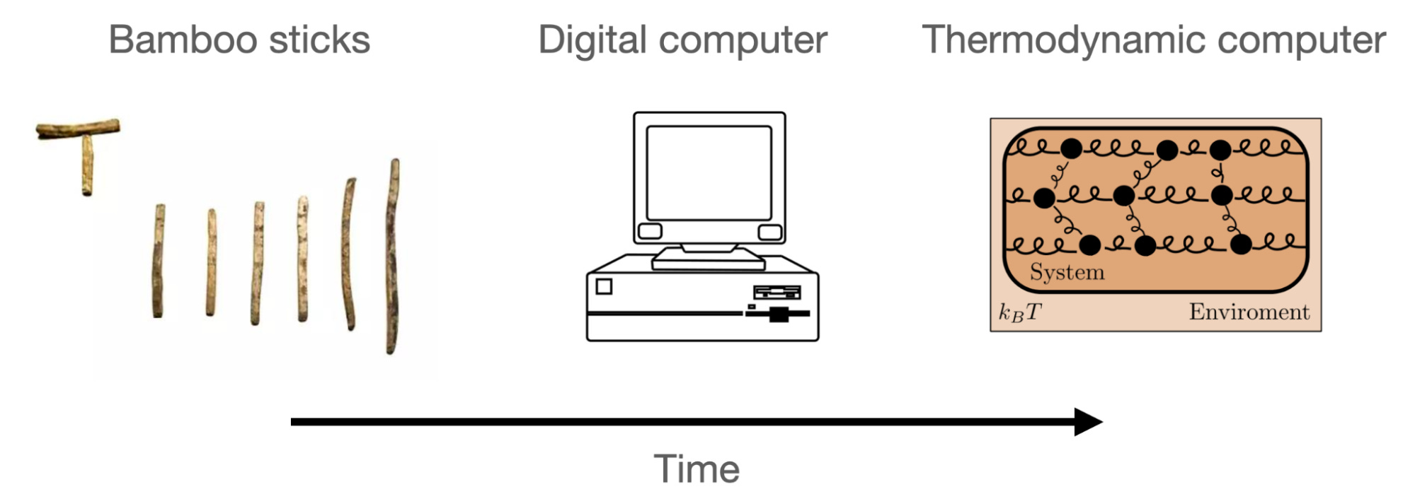
Nowadays agriculture is just one of many places where linear systems appear. The applications for linear algebra problems have multiplied over the years, and so have the means of solving them. Homo Sapiens, as a species, has a reputation for its innovative use of tools, and, in a way, the tools used in different times even define the eras of civilization. Bamboo rods worked well for linear systems with only a few unknown quantities, but quickly became impractical as the number of variables grew.
The standard method used to solve linear systems with counting rods seems to have been equivalent to Gaussian elimination, meaning the number of steps in the calculation was proportional to the cube of the number of variables. Currently, the state-of-the-art tool is a digital computer with a Graphics Processing Unit (GPU), a chip which is specifically designed to quickly perform linear algebraic operations. Instead of using Gaussian elimination, other algorithms are available (such as conjugate gradients) to be run on the GPUs which only require a number of steps proportional to the square of the number of variables, a great improvement over the ancient methods.
Linear algebra in machine learning
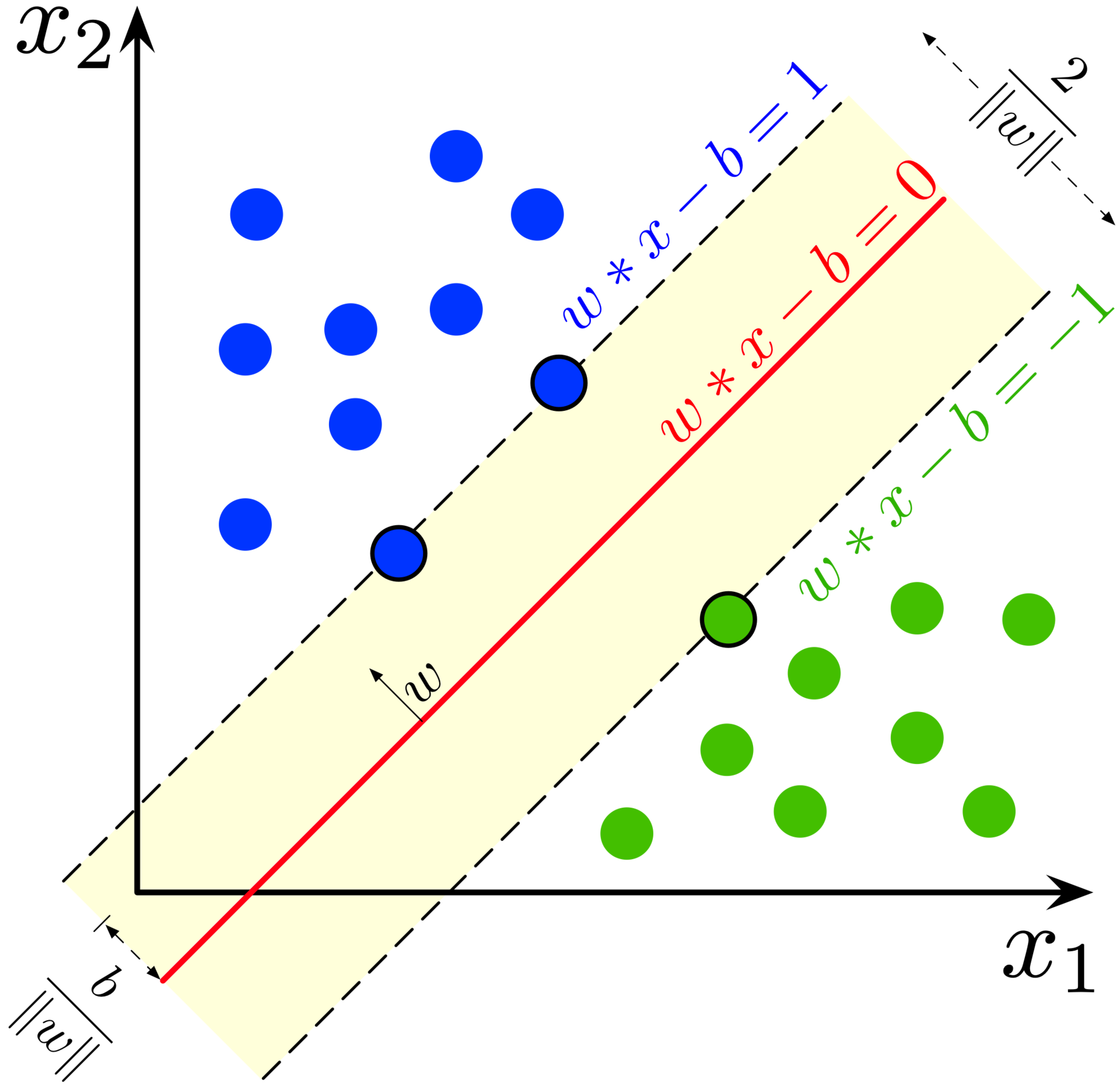
One area where GPUs have massively contributed to accelerating linear algebra primitives is machine learning. One of the many examples of solving a linear system of equations in machine learning is in support vector machines. There, one must find the hyperplane that best separates two classes of features. Below is a figure where the plane corresponding to the solution of the linear system is shown, that best separates blue and green sets of points which are often extracted features of a dataset.
Another example is Gaussian process regression (GPR), which is an important algorithm that includes uncertainty estimates. In GPR, one must invert the kernel matrix to obtain the mean and covariance of the posterior probability density function. There, matrix inversion is one of the more costly subroutines of the algorithms. A third linear algebra primitive we focus on in our paper is estimating the determinant, which is also an important subroutine in Bayesian learning.
Evolution of hardware
What our paper is about is a new physics-based tool for solving linear-algebraic problems, along with new algorithms to use with it. This physics-based system can be viewed as a thermodynamic computer.
The thermodynamic computer
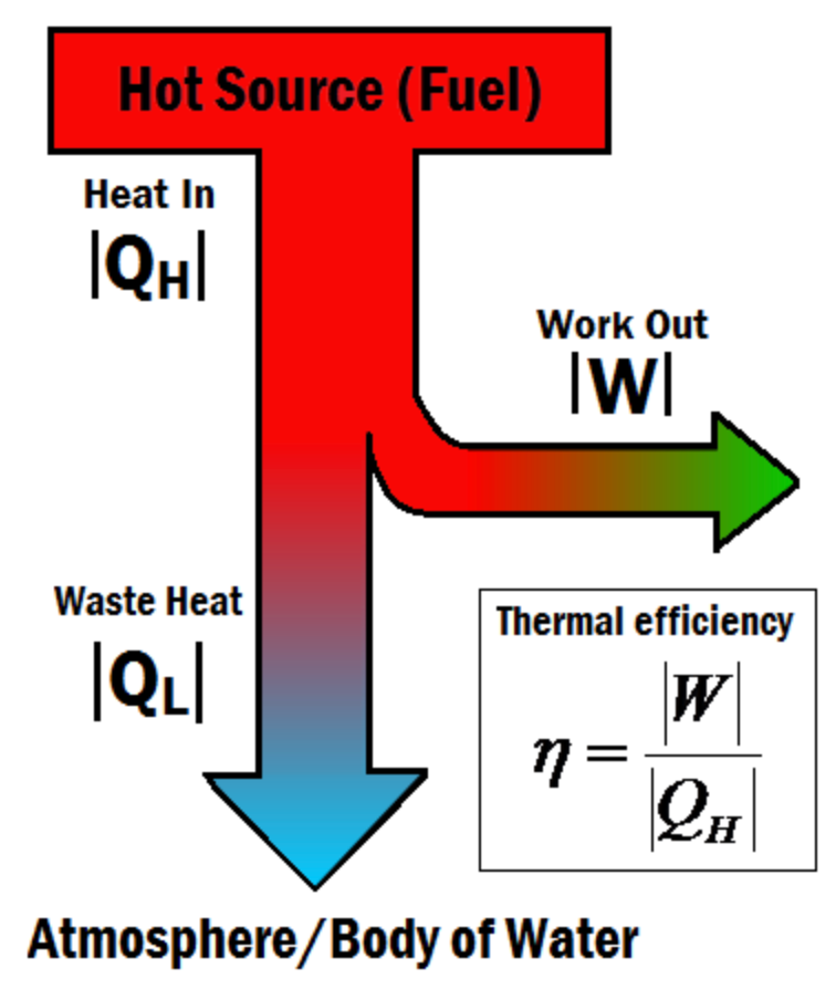
Thermodynamics is often called a theory of work and heat, which it is. But as conceived by its “father” Sadi Carnot, it was a theory about steam: in particular, of how to harness its power, to capture steam in a piston and use it to drive hulking locomotives across Europe. The subject does not find its origins in intellectual curiosity, and definitely not in a philosophical investigation of time’s arrow, but in the need to solve a practical problem. For this reason, thermodynamics has a different flavor than other physical theories, because it is more about how a system responds to a procedure conducted by an external operator, rather than the behavior of the system in isolation. As Herbert Callen writes in Thermodynamics and an introduction to thermostatistics:
The single, all-encompassing problem of thermodynamics is the determination of the equilibrium state that eventually results after the removal of internal constraints in a closed, composite system.
In fact, much of the theory can be interpreted as relating the inputs and outputs of a system undergoing an engine cycle, which is a sequence of operations that are performed on the system, one after another. Consider, though, that a sequence of operations performed on a device, resulting in a particular relation between its inputs and outputs, is nothing other than an algorithm. In other words, thermodynamics is the study of physically realized algorithms operating on macroscopic systems.
How, then, do we design a thermodynamic device to implement algorithms that are useful? One way is to use the minimum energy principle: that a system in thermal equilibrium with its surroundings is in a macroscopic state where the energy is minimized with respect to all external constraints on the system (including temperature). If the microscopic state of the device is described by a vector of coordinates x and the potential energy of the system is given by a function V(x), then at thermal equilibrium the coordinate vector x is a random variable, whose density function is the Boltzmann distribution
where Z (the partition function) is a normalization factor. Then we need only engineer the potential energy V(x) such that this equilibrium distribution somehow contains the solution to the problem we would like to solve. Suppose that we take a potential energy function of the following form
where the (positive definite) matrix A and vector b are chosen by the user. In this case, the Boltzmann distribution is a normal distribution, or Gaussian
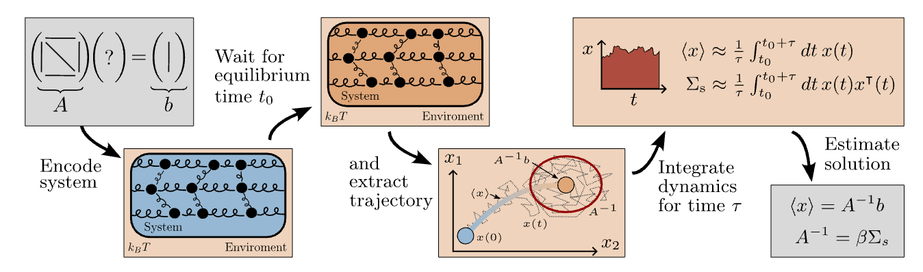
The mean of this distribution is the solution to the linear system Ax = b. We also see that the covariance matrix is proportional to the inverse of the matrix A. Using these two facts, we can devise a protocol for solving linear systems and inverting matrices based on the thermodynamics of this system, which physically corresponds to a set of harmonic oscillators that are coupled to each other.
The method is illustrated in the figure below. One simply sets the matrix A and vector b to those appearing in the equation Ax = b, then, after waiting for equilibration, one can average the value of the vector x over time using, for example using an electrical circuit, where the components of x might be the voltages at different points in a circuit. This average will be the solution of a linear system, and similarly the covariance matrix of x can be estimated by an analog device.
While it may be interesting in an academic way that this is possible, it is not immediately clear that there is any reason to attempt to solve these problems using networks of coupled oscillators, especially given that the SOTA GPUs are so effective. Remarkably, the simple method described above can be theoretically shown to be more efficient than existing digital methods in the limit of a large number of variables.
Achieving thermodynamic advantage
Thermodynamic speedups
Efficient ways to solve linear algebra problems were largely discovered in the 20th century, motivated by the need to solve larger problems with the limited hardware available at the time. These include, for example, the conjugate gradient method for solving linear systems and the Cholesky decomposition, which can be applied to linear systems, matrix inversion, and other problems. Even with these methods, the demand grew for faster and faster calculations; the live rendering of the three-dimensional environments needed for modern video games was especially taxing, spurring the invention of the GPU. Modern GPUs accelerate the evaluation of linear functions significantly, but the number of algorithmic steps needed to solve a linear system of equations has remained asymptotically proportional to the square of the number of variables, while inverting a matrix has required a cubically-growing number of steps.
This is often expressed using big O notation. When we write that a runtime is in O(d), it means that the runtime scales linearly with dimensionality, omitting any prefactors in what the actual runtime is, that can depend on other factors such as parallelization.
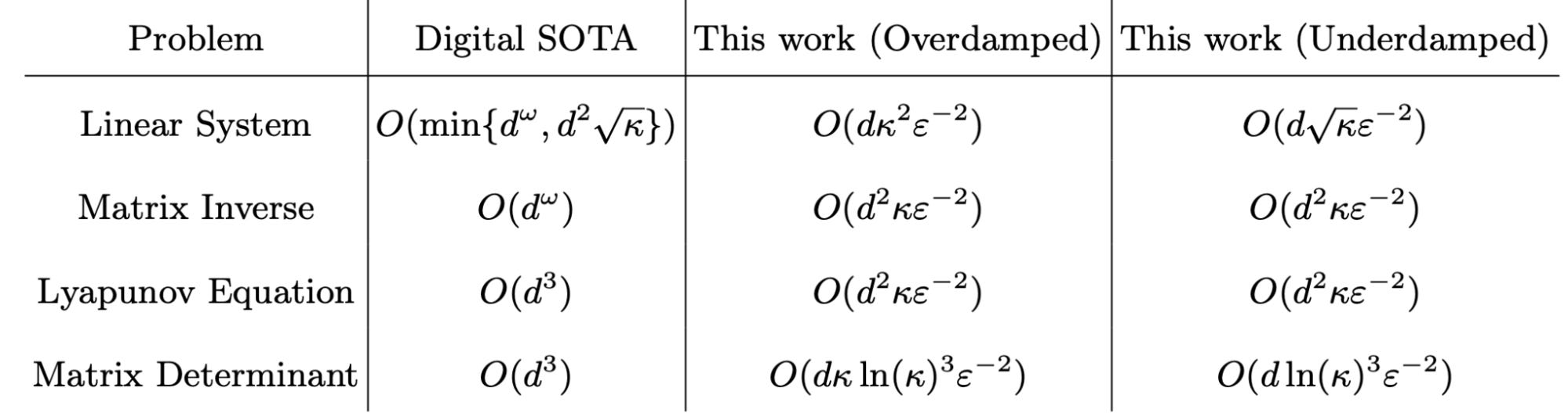
The thermodynamic algorithm for solving linear systems outlined previously takes advantage of the physical equilibration process in the hardware, which can be thought of as performing matrix-vector multiplications in constant time. This enables us to prove that a linear system of equations can be solved in an amount of time proportional to the number of variables using a thermodynamic computer. We derived similar algorithms for solving other common problems in linear algebra: inverting a matrix, solving the Lyapunov equation, and evaluating the determinant of the matrix. In each case, the asymptotic time-complexity of the thermodynamic algorithm is better than the best known digital algorithm by a factor on the order of the number of variables, which can probably be explained as stemming from a constant-time matrix-vector multiplication achieved by the hardware.
Time and energy
It could be argued that the number of steps taken by a digital algorithm is not the right metric, given that these algorithms may be parallelized sometimes, so the physical time necessary is not limited by the number of elementary operations. Another cost of computation is the necessary energy expenditure though, which should also be taken into account. If parallelizing an algorithm across two processors decreases the time, it may also increase the energy, so the product of energy and time is of special importance. The thermodynamic algorithm for solving a linear system has energy-time product scaling with the number of variables, whereas all existing digital algorithms we are aware of have energy-time product scaling with at least the square of the number of variables. Our paper gives the energy-time complexity for solving linear systems is as
where d is the number of variables, κ is the condition number of A (its largest eigenvalue divided by its smallest eigenvalue), and the other quantities are physical constants and tolerance parameters specifying the degree of accuracy of the solution.
Harder, better, faster, stronger
We’ve reached a milestone in this story–the thermodynamic computer is a new piece of hardware that can solve linear algebra problems faster than conventional digital computers, under mild assumptions. Will there be further progress, or is this paradigm the optimal model of linear algebraic computation? It is easy to imagine a future in which incremental improvements in efficiency continue, relegating the thermodynamic computer to the hardware graveyard alongside bamboo counting rods. But underlying this question is a deeper one about the fundamental hardness, or complexity, of solving the problem at hand. It is relatively straightforward to prove that a particular problem can be solved with an amount of resources limited by some upper bound; one must simply provide the algorithm. But lower bounds on computational hardness are far more elusive, and finding such bounds remains a sticking point of computational complexity theory.
In thermodynamics, proven lower bounds on the resources necessary to accomplish some task are commonplace, for example the minimum energy which must be dissipated in order to produce a certain amount of work from two heat reservoirs is the seminal result of Carnot’s study of engine efficiency. In fact, thermodynamics is the only branch of physics where we have a definite notion of irrecoverable cost, and the general format of these results is that to do a given thing in a shorter period of time, one has to spend more energy. So, perhaps, the thermodynamic computing paradigm can shed light on the complexity of computations. This idea goes hand in hand with the study of optimality for thermodynamic algorithms. In calculating the efficiency of his engine cycle, Carnot found that this result was not just relevant to steam engines, but in fact was a general limit on the efficiency of any device which produces work from heat. Similarly, we conjecture that the limit we have found on energy and time costs may be generalizable to other models of computation. Because our results can be stated in terms of the energy-time product necessary for a computation, it is natural to investigate whether thermodynamic algorithms exist that achieve a lower energy-time product (in which case our algorithms would not be optimal), or otherwise to prove that none exist.
This line of thinking connects to the “mortal computation” advocated by Geoff Hinton (which inspired the title of this post). While cutting-edge artificial intelligence algorithms consume great quantities of energy, it is not known whether they may be carried out at reduced cost, and to what extent, by analog hardware that offloads some or all of the algorithm to naturally-occurring physical processes. It seems important, then, to ask whether thermodynamic formulations can identify the optimal efficiencies of AI algorithms, and ultimately provide protocols for achieving optimal performance.
Speedups: in practice
You may also be curious of what speedups we can actually get in practice, other than bounds, that may not be tight and which put aside prefactors. To investigate this, we compared our method’s performance by measuring the error obtained by running it on ideal hardware (with no imperfections, that we leave for future work) to the performance obtained for other digital methods. To solve linear systems, the conjugate gradient method and the Cholesky decomposition are used. We also estimated the runtime of the thermodynamic hardware by constructing a timing model that takes into account all the operations involved to obtain a solution, such as digital-to-analog and analog-to-digital conversions, and other digital overhead. This model is based on an RC circuit implementation that only involves passive electrical components, and is discussed in the next section. The results are that even for modest dimensions (around 1000) and condition numbers, we obtain solutions competitive to conjugate gradients. We see that this advantage grows with dimension, as expected from the analytic bounds we obtain. We also see that by lowering the temperature, even better results can be obtained, hence showing the thermodynamic nature of the device.
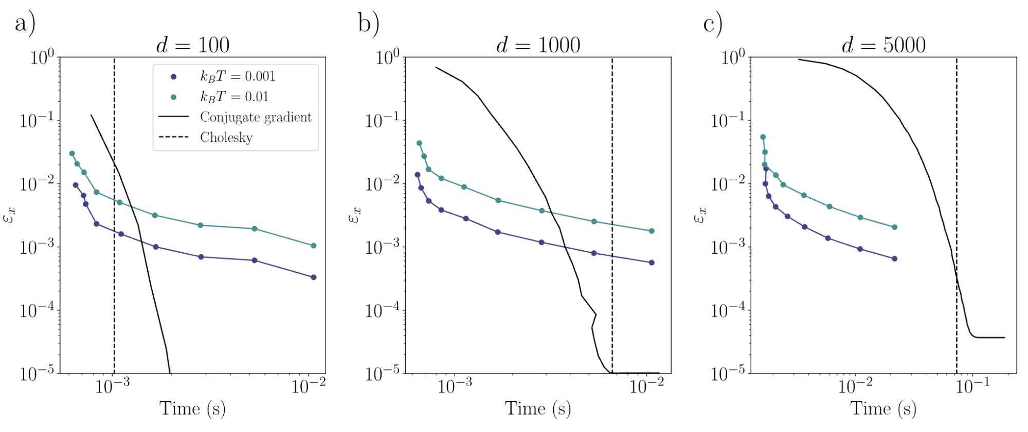
This is even more exciting, as it shows that a simple thermodynamic hardware proposal can yield speedup advantages for simple problems for which GPUs were optimized for. Hence we expect this to be optimized a lot in the future.
A potential hardware realization
The discussion up to this point may seem very abstract–what does a thermodynamic computer actually look like “in the flesh”? Below is a circuit diagram of one possible implementation of a single component (or cell) of the thermodynamic computer, taken from our previous work (see also this talk).
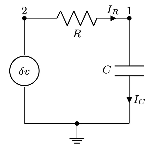
To solve a linear system that has d variables, d of these cells would be needed, with each cell coupled to all the others (for d² total connections). A single cell contains a resistor and a capacitor, and a noise source in series (the resistor also produces voltage fluctuations due to Johnson-Nyquist noise at finite temperature, which may be effectively included in the noise source). There is also a constant DC bias applied to each cell, which encodes the components of the vector b. The entries of the matrix A are encoded in the couplings between cells, which may be either resistive or capacitive. Of course this is just one possible version of the thermodynamic computer; recall that the definition of the device is at the level of the potential energy function V(x), and the vector x may represent essentially any measurable physical degree of freedom. As all physical systems have energy functions (Hamiltonians), this is a very general level of description, which could be applied, for example, to engineering similar models with optical hardware.
We thank you for taking the time to read this blog!
A bright future
At the core of Normal Computing’s mission is bridging artificial intelligence, particularly generative AI, to high stakes enterprise decision-making applications. We are approaching these problems with a mix of interdisciplinary approaches across the full stack, from hardware and physics to software infrastructure and algorithms. Future physics-based hardware may allow for a step change in AI reliability and scale, in part by admitting new co-developed algorithms. If you are interested in pushing the boundaries of reliability in AI with us, get in touch at info@normalcomputing.ai!